A Review of Different Interpretation Methods (Part 1: Saliency Map, CAM, Grad-CAM)
In order to build trust in machine learning models and move towards their integration into our everyday lives, we need to make “transparent” models that could explain why they predict what they predict. To this end, many researchers have proposed several methods that help us gain insights into how these “black-box” models work. In this post, I will go through some of the most frequently used interpretation methods in deep learning, one of the fruitful areas of research in machine learning. As plenty of interpretation methods exist, I will cover only those that are applied to image classification neural networks in this post, and leave the other methods for separate posts. The techniques covered in this article include Saliency maps, CAM, and Grad-CAM.
Before going into any details, it is helpful to get an overall picture of interpretation methods and how they work by trying to categorize them. The following three categorizations are the most common ones found in the literature:
- Categorizing based on locality:
- Local methods: Local methods explain the predictions of a model by investigating its performance on a specific set of examples. For instance, you can feed an image (or a collection of images) of a human’s face to a classifier network and probe if the model uses the right cues in the image (e.g., nose, lips, eyebrows, etc.) to come up with the correct prediction.
- Global methods: In contrast to local methods, global methods can explain how a model works even without probing its functionality on a specific set of inputs. As a simple and concrete example, let’s suppose that we have a linear regressor that can predict the price of a house based on the longitude and latitude of it (I know that it would be a terrible regressor, but it can vividly demonstrate my purpose). So, the model consists of a tuple of weights (w1, w2) — let’s forget about the bias term here — and its prediction of the price would be w1×longtitude+w2×latitude. Now let’s suppose that in our model w1 >> w2. Therefore, the regressor obviously outweighs longitude to latitude, or in other words, longitude is a much more important feature than latitude for predicting the price. As you might have noticed, I just provided a simple global explanation of how our (bad!) regressor works without feeding any data points to it.
2. Categorizing based on specificity:
- model-specific: As its name suggests, a model-specific method can only be applied to a specific group of models. Considering our linear regressor again, what I did was to just compare the weights of the model, as measures of the importance of features, which is completely intuitive. However, this approach would not work for feed-forward neural networks as there are lots of nonlinearities in between the features as the input to the model, and the predictions as the output of the model. Thus, the simple explanation that I provided just holds for linear regressors and might not hold for a more sophisticated model.
- model-agnostic: A model-agnostic explanation method can be applied to any machine learning model. When we use such a method, the model is seen completely as a black-box function and no information about the internal structure of the model is required. What we just need to know is that the model is a function that gives an output for each valid input it gets.
3. Categorizing based on the direction of the flow of interpretation signal (don’t bother if the term “interpretation signal” does not make sense to you as I made it up by myself! you will understand what I mean by that if you keep reading the article):
- Gradient-based backpropagation methods: Methods that backpropagate an importance signal from the output towards the input. In fact, we start from the output of the network and assign an importance score to each intermediate value computed during the forward pass. A score function based on the gradient of output w.r.t each intermediate value, which can be calculated easily with the backpropagation algorithm, could be a reasonable choice and can show us how changing that part would affect the output. Thus, these methods can be called “gradient-based” methods.
- Perturbation-based forward propagation methods: Methods that perturb the input and probe its possible effects on the prediction of the network. For example, by occluding some part of the input image and investigating the changes in the output, we can understand how that part contributes to the network’s prediction. In contrast to backpropagation methods, we need to use a forward pass to transfer the changes in the input to the scores that are computed by the very last layers.
Now let’s go through the details of the interpretation methods:
1. Saliency maps
Saliency map is an explanation method used for interpreting the predictions of convolutional neural networks (CNNs). This is probably the oldest and the most frequently used method of interpretation in deep learning. Basically, the saliency map of an input image specifies parts of it that contribute the most to the activity of a specific layer in the network, or the decision of the network as a whole.
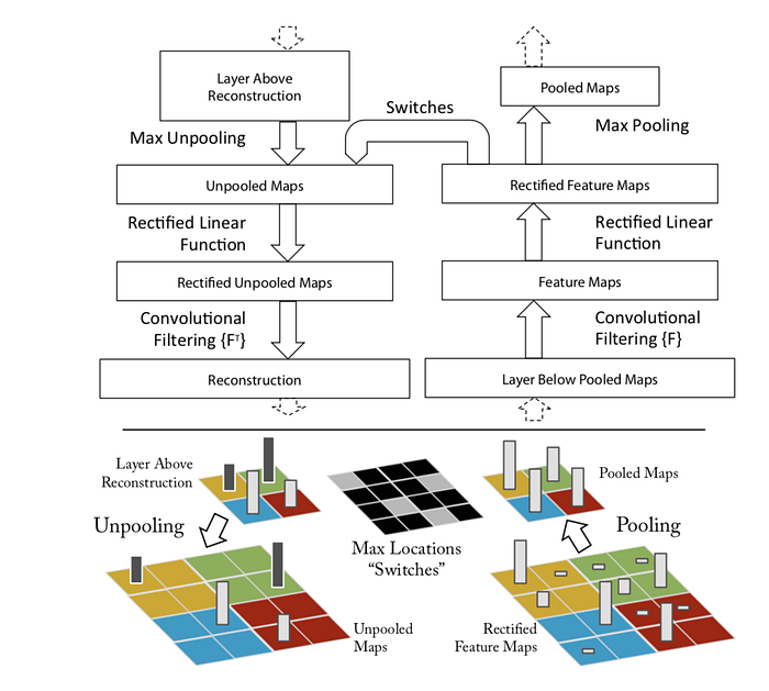
There are three main approaches to getting the saliency map of an input image for a CNN. The first proposed approach is using deconvolutional networks introduced by [Zeiler and Fergus 2013]. In this paper, to recognize which features (which are basically the pixels) in the input image an intermediate layer of the network is looking for, the authors have proposed a deconvolutional network that reconstructs the input from the activation of that layer. In order to do that, the operations done in between the input and that particular layer are inverted. More specifically, deconvolution is used as the inverse of convolution (with the transposed version of the same filters), unpooling is used as the inverse of pooling, and ReLU is used as the inverse of itself, but clamping the negative values of the signal going backward from the activation space to the image space. It is worth noting that as the pooling operation is non-invertible, the authors have used a module called switch in the deconvolutional network to recover the positions of maxima in the forward pass. The whole process can be depicted as in the following figure:
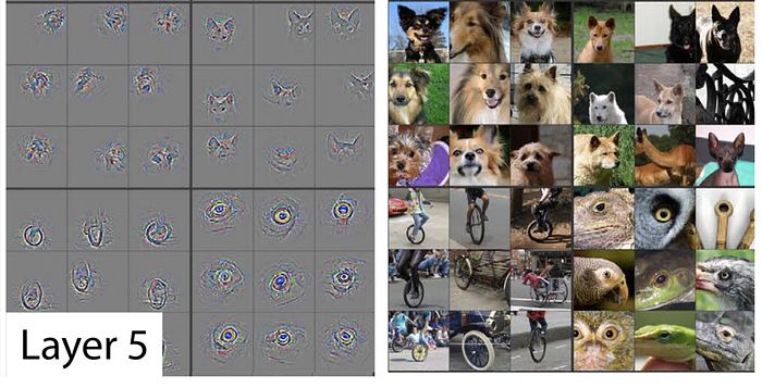
Here are some of the results of the reconstruction of the input image from the activations of the fifth layer of ZFNet:
The second and probably the most straightforward approach of getting a saliency map is using the backpropagation algorithm to compute the gradients of logits wr.t. to the input of the network (note that in the backpropagation algorithm used for training the network, the gradients are computed w.r.t. the parameters of the network). This approach was first proposed by [Simonyan et al. 2013]. Using backpropagation, we can highlight pixels of the input image based on the amount of the gradient they receive, which shows their contribution to the final score:
[Simonyan et al. 2013] has also shown that the backpropagation method is quite similar to using deconvolutional networks, but with one major difference; in the deconvolutional network, ReLU clamps the backward signal — coming from activation of the intermediate layer — if the backward signal itself is negative, while the backpropagation method clamps the backward gradient if the input of the ReLU through the forward pass was negative.
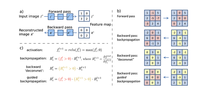
[Springenberg et al. 2014] combined these approaches and proposed the guided backpropagation algorithm as the third way of getting saliency maps. In fact, instead of masking the importance signal based on the positions of negative values of the input signal in forward-pass (backpropagation) or the negative values of the reconstruction signal flowing from top to bottom (deconvolution), they mask the signal if each one of these cases occurs. The following figure depicts the guided backpropagation algorithm very well:
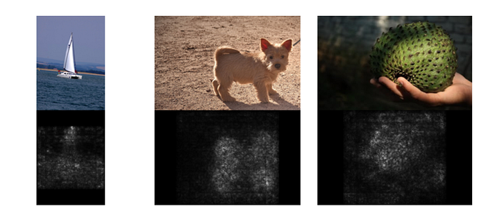
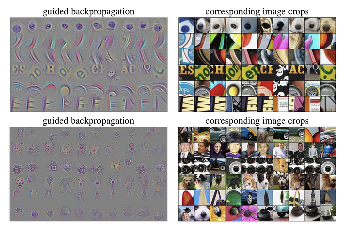
Here are some of the saliency maps produced by the guided backpropagation method. As can be seen — and reported in other works too — , this algorithm is quite good at capturing high-resolution and sharp saliency maps:
It is pretty straightforward to check that the saliency map is a local gradient-based backpropagation interpretation method. Although saliency maps are mostly used for interpreting CNNs, However, as the concept of gradient exists in all neural networks, one can use it for any arbitrary artificial neural network. Thus, it could be considered as a model-agnostic interpretation method.
Finally, it is worth noting that there a couple of papers that have shown saliency maps are not always reliable. [Kindermans et al. 2018] demonstrate that data preprocessing, such as subtracting the mean and normalization, can make undesirable changes in saliency maps. [Ghorbani et al. 2019] also show that saliency maps are vulnerable to adversarial attacks.
2. Class Activation Mapping (CAM) and GRADient-weighted Class Activation Mapping (Grad-CAM)
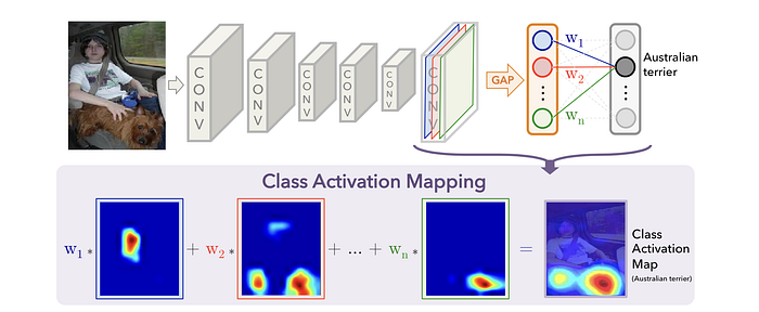
Class activation map (CAM) is another explanation method used for CNNs, introduced by [Zhou et al. 2016]. The authors of the paper have evaluated networks with the architecture similar to the Network in Network’s architecture. In these networks, the stack of fully connected layers at the very end of the model has been replaced by a layer named Global Average Pooling (GAP). GAP simply averages the activations of each feature map and concatenates these averages and outputs them as a vector. Then, a weighted sum of this vector is fed to the final softmax loss layer. Using this architecture, we can highlight the important regions of the image by projecting back the weights of the output on the convolutional feature maps. The following figure illustrates this process:
Grad-CAM is a more versatile version of CAM that can produce visual explanations for any arbitrary CNN, even if the network contains a stack of fully connected layers too (e.g. the VGG networks).
In order to get the Grad-CAM of a given image and a class of interest, we can take a quite similar approach to what we took in computing saliency maps; we let the gradients of any target concept score (logits for any class of interest such as ‘human’s face’) flow into the final convolutional layer. We can then compute an importance score based on the gradients and produce a coarse localization map highlighting the important regions in the image for predicting that concept.
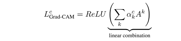
More formally, at first, the gradient of the logits of the class c w.r.t the activations maps of the final convolutional layer is computed and then the gradients are averaged across each feature map to give us an importance score
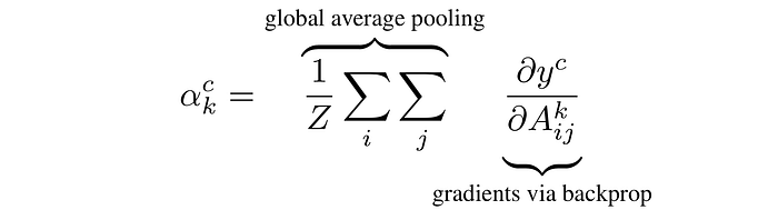
Where k is the index of the activation map in the last convolutional layer, and c is the class of interest. Alpha computed above shows the importance of feature map k for the target class c. Finally, we multiply each activation map by its importance score (i.e. alpha) and sum the values. To only consider the pixels that have a positive influence on the score of the class of interest, a ReLU nonlinearity is also applied to the summation:
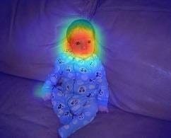
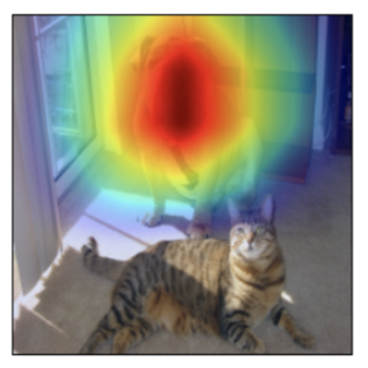
The following figure shows a visualization produced by GRAD-CAM:
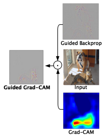
As Grad-CAM can only produce coarse-grained visualizations, the authors have also combined guided-backpropagation with their method and propose Guided Grad-CAM. They simply do that by an element-wise multiplication of guided-backpropagation visualization and Grad-CAM’s visualization:
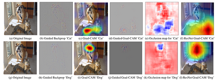
Here are some more examples of visualizations of the methods introduced above:
CAM and Grad-CAM and their variants are all local backpropagation-based interpretation methods. They are model-specific as they can be used exclusively for interpretation of convolutional neural networks.
